OWASP FSTM, stage 3: Analyzing firmware

Analyzing a firmware dump is not a simple task that can be summarized in simple steps to obtain a formula valid for all cases. Different techniques that can help extracting data from these dumps will be reviewed down below.

It is common during firmware analysis to be confronted with undocumented formats, proprietary solutions, and even encrypted data. For this reason, it is important not to lose the context in which the analysis is performed and to consider all the information gathered in the previous steps. With this context in mind, it will be possible to make a judicious choice between the various tools and techniques here proposed for analyzing firmware.

Next, it is proposed to transform the available firmware dump format into a standardized binary format for further analysis. A section is also dedicated to those cases in which our firmware may include more data than desired, which may alter the results of subsequent tests. Finally, metrics, tools and techniques that allow us to identify sections, formats and signatures within a firmware for later extraction are listed.

Obtaining a raw binary dump

Depending on the techniques used in step two (OWASP FSTM, stage 2: Obtaining IOT device firmware) of this guide, the firmware dump may be in different formats. The goal of this section is to convert that format into a raw binary format.

Many of the analysis tools available, will be based on binary formats and obtaining a binary is an important task in case at some point you want to perform a full emulation of the device.

In this first step, it relies on previous information to know in which format the firmware dump has been performed. The researcher must consult the documentation of the tool used to be sure to perform a conversion to binary format.

However, a text editor and hexadecimal editor should be sufficient to verify the information of the tools used or to find out in which format a dump can be found. The following is a summary of the most common formats for this type of task and their typical characteristics.

Intel HEX

Being one of the oldest formats for representing the contents of memories, it can be characterized by its line start code, the colon ‘:’. Although the format is more complex, for simple cases it can be summarized in that for each line it usually includes the start code, a record length, the record address, a record type (data, usually) and a final checksum. More details on the format can be found at the following link. To obtain a binary from such a file, multiple tools can be used such as Intel_Hex2Bin, or SRecord.

:10010000214601360121470136007EFE09D2190140
:100110002146017EB7C20001FF5F16002148011988
:10012000194E79234623965778239EDA3F01B2CAA7
:100130003F0156702B5E712B722B732146013421C7
:00000001FF

SREC or Motorola S-Record

This format is like Intel HEX. Again, a start code is defined along with different fields to describe data records in hexadecimal format. It can be distinguished because in this case the start code is an ‘S’. More information can be found at this link. To convert this format to binary, the same tools can be used as in the previous section.

S00F000068656C6C6F202020202000003C
S11F00007C0802A6900100049421FFF07C6C1B787C8C23783C6000003863000026
S11F001C4BFFFFE5398000007D83637880010014382100107C0803A64E800020E9
S111003848656C6C6F20776F726C642E0A0042
S5030003F9
S9030000FC

Hexdump or hexadecimal string

As discussed in the article OWASP FSTM, stage 2: Obtaining IOT device firmware, sometimes you will have access to devices through text interfaces and with limited tools. One of the most common options in this case for memory dump is hexdump or one of its alternatives. Normally a hexdump with these tools consists of an address column, a column with the memory contents in hexadecimal and finally an optional column with the contents encoded in text. To restore this format to a raw binary one of the most common tools is xxd with the ‘ – r’ parameter of revert. For more information about the format see the following link.

00000000 30 31 32 33 34 35 36 37 38 39 41 42 43 44 45 46 |0123456789ABCDEF|
00000010 0a 2f 2a 20 2a 2a 2a 2a 2a 2a 2a 2a 2a 2a 2a 2a |./* ************|
00000020 39 2e 34 32 0a |9.42.|

Base64

As with hexdump, base64 is a useful format for transmitting an encoded binary over a channel that only supports printable characters. Although it is less common to find a utility to generate the base64 of a file, many modern languages include libraries to do so.

If an embedded device is found without a command line utility for base64, it is common to be able to encode from Python, Perl or other languages on the device. Base64 defines a table that allows to transform between a binary value and a map defined for this encoding. The advantage is that this table of values, instead of being of 16 symbols (hexadecimal) is of 64, allowing to contain much more information for each character transmitted, saving a lot of bandwidth in communications very limited in speed. Because this encoding includes more than one byte per symbol, it sometimes requires a final padding that is done with the character ‘=’, very characteristic of this representation. To learn more about this encoding, see the following link.

bGlnaHQgd29yaw==

Out-of-band and parity data screening

Once you have a binary file it is time to remove the out-of-band and parity data to get only the exclusively useful portion of the memory.

The out-of-band data in flash memory is used to store an index of memory blocks that are in bad condition to avoid their use. A bit pool for parity calculation is also usually included in this section so that there is a mechanism for detecting faults and correcting the bits that may have caused the error.

This step is only relevant after a memory dump using “chip-off” techniques, which consist of the physical extraction of the memory, since, in these cases, all its contents are extracted, including sections used as redundancy to improve the integrity of the stored data.

The example case is a NAND Flash memory dump.

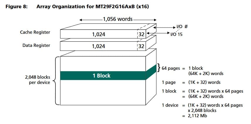
Source: Micron

As can be seen in the image above, taken from the datasheet of a Micron NAND Flash memory, this memory is organized in blocks. Each of the 2,048 blocks has a set of 64 pages. According to the image, for this memory, each page is 1,024+32 words wide. When the user accesses the memory, he perceives that each page occupies a total of 1,024 words, although in the memory structure there are 32 additional words that serve for memory error correction.

This example structure is quite common, although each manufacturer may choose varied sizes for these redundancy structures or even other arrangements where the redundant memory is in blocks at the end of the memory instead of being interleaved within each block or page.

For the analysis and elimination of redundant data in a dump there are solutions that attempt to automate the process such as https://github.com/Hitsxx/NandTool, although sometimes a manual analysis will have to be performed by studying the entropy of the file and even autocorrelation techniques.

Once a file has been obtained in binary format without redundancy or “out of bands” data, the process of analyzing the firmware contents begins.

Entropy analysis

Computational entropy is a concept from information theory, developed by C. E. Shannon, which attempts to obtain a measure of the uncertainty of the possible values that a random variable can take. For a data set of indeterminate origin and format, this concept has been reinterpreted to try to obtain a measure of the randomness of the values it contains.

Because of the change of context in which the concept of entropy is applied, the results of the calculation for a data set of indeterminate structure are closer to a measure of how much the bytes in the sample vary.

Based on this definition, the utility of the concept in the study of a firmware image is shown below.

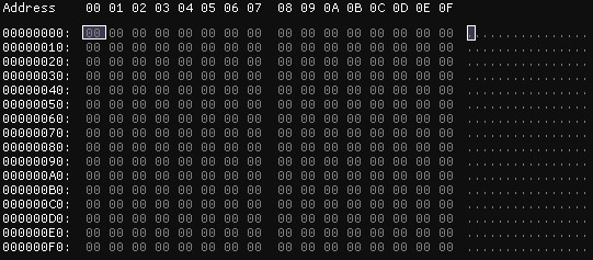
Using an (assumed) random generator, a 256-byte file is generated as shown in our image (all generated numbers are 0). Since there is no randomness in the values, the total entropy of the file is 0.

Using the second definition, it can be understood that, since there is no variation among the bytes, the entropy calculation is 0.

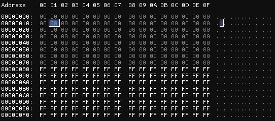
If the programmer has “corrected” the random generator used in the previous example, another 256 bytes of information are dumped into a file, this time the result is that half of the file contains the value 00 and the other half contains the value FF. In this case, the file contains more “randomness” than in the previous case, so an increase in this measure is expected. To verify this, binwalk is run in entropy calculation mode and the result is higher than in the previous case, 0.125.

% binwalk -E halfceros.bin

DECIMAL HEXADECIMAL ENTROPY
——————————————————————————–
0 0x0 Falling entropy edge (0.125000)

It should be noted that some of these tools “normalize” the calculated entropy value. Some tools will give a value of 1 entropy point out of a maximum of 8, while others will show a value of 0.125 out of a maximum of 1.

It could also be said that the bytes in this file vary somewhat more from each other than in the previous case.

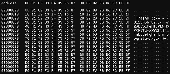
Continuing with the previous example, if the random generator now writes all possible values of a byte sequentially in our file, the entropy is triggered to its maximum. If the information source is random, that information source can use all bytes so its “randomness” is high.

% binwalk -E fullent.bin

DECIMAL HEXADECIMAL ENTROPY
——————————————————————————–
0 0x0 Rising entropy edge (1.000000)

This is a clear example of taking entropy as an accurate measure of randomness is a mistake. In this case, the randomness of the content is low, and the next value could be predicted by simply adding one unit to the previous value. In this case, it should be understood is that the bytes have the maximum possible variation, as each one takes a different value from the previous ones.

A more mundane example of this could be given with our language. Taking as a symbol a word instead of a byte, if you analyze the entropy of a literary work, you will get an unknown entropy value X.

If in this same work all pronouns were removed, we would still be able to understand it in its entirety. The pronouns, while frequent, provide little information within the literary work. If we were now to perform a calculation of the entropy of the work without the pronouns, we would find a larger Y-measure than in the previous case (Y>X).

The example reveals that each word in the second work provides more information on average than in the first, even though in neither case has the choice of words been completely random.

To expand on this concept, we recommend reading the Wikipedia article.

In the case of firmware analysis, entropy analysis can help identify signatures and give clues to different data sources.

Since the data being analyzed is not completely random, entropy analysis can be used to identify different origins of this data.

If the entropy of the firmware file of our device is calculated in moving windows, a continuous measure of the entropy of the file will be obtained and can be represented graphically. This plot can be continuous or have a high variance and this can tell us that the data being observed may come from different algorithms or have different uses.

To exemplify this, an analysis is performed on the OWASP “IoT Goat v1.0” image. This is a deliberately vulnerable image for the study of these techniques and can be found at this link.

An entropy calculation is performed on this firmware image:

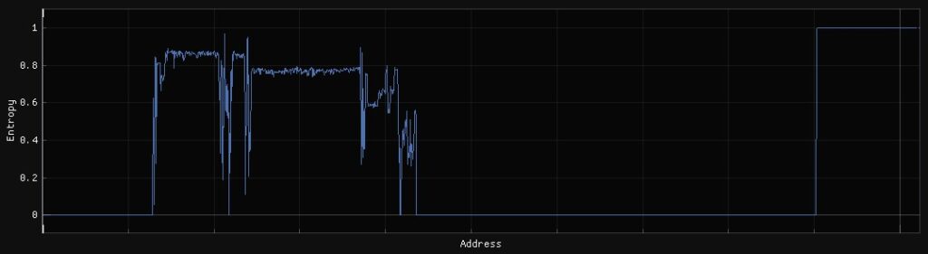
From this image it can be extracted that there are possibly several sections with various uses in this firmware. There appears to be an initial section with no content followed by a section with high entropy. In the middle there are parts with various peaks that would need to be analyzed in more detail, but then there is another flat section with another level of entropy lower than the first. This could look like another file type, format, or firmware partition.

After this section is another turbulent and unclear area, followed by a large valley that seems to have no use and finally an area of very high entropy that is possibly a third section.

The points where these entropy variations occur are important study points. In them it is possible to find signatures of formats or algorithms used to generate them.

In addition to the information provided by the entropy variation, its value allows us to make assumptions about the state of the data.

In sections where high entropy values are found, it is due to the use of data compression or encryption algorithms. Compression processes generate the highest entropy values as they attempt to pack as much information as possible per byte, while encryption processes, which seek to maximize the randomness of the result, are usually just below compression. This may not be true for all compression and encryption algorithms.

Signature identification

File formats and file systems use a series of bytes as identifiers, usually called “magic numbers” or signatures. During firmware analysis it is especially useful to identify signatures of known file types, for which multiple tools are available.

The most used automatic tool for analyzing firmware is binwalk. It has functions for identifying files in the firmware, both by searching for signatures and by detecting the coding of a section and looking for patterns. The basic use of binwalk is through the terminal:

$ binwalk IoTGoat-raspberry-pi2.img

DECIMAL HEXADECIMAL DESCRIPTION
——————————————————————————–
4253711 0x40E80F Copyright string: “copyright does *not* cover user programs that use kernel”
…
4329472 0x421000 ELF, 32-bit LSB executable, version 1 (SYSV)
4762160 0x48AA30 AES Inverse S-Box
4763488 0x48AF60 AES S-Box
5300076 0x50DF6C GIF image data, version “87a”, 18759
5300084 0x50DF74 GIF image data, version “89a”, 26983
…
6703400 0x664928 Ubiquiti firmware additional data, name: UTE_NONE, size: 1124091461 bytes, size2: 1344296545 bytes, CRC32: 0
…
6816792 0x680418 CRC32 polynomial table, little endian
6820888 0x681418 CRC32 polynomial table, big endian
6843344 0x686BD0 Flattened device tree, size: 48418 bytes, version: 17
6995236 0x6ABD24 GIF image data, version “89a”, 28790
…
12061548 0xB80B6C gzip compressed data, maximum compression, from Unix, last modified: 1970-01-01 00:00:00 (null date)
12145600 0xB953C0 CRC32 polynomial table, little endian
12852694 0xC41DD6 xz compressed data
12880610 0xC48AE2 Unix path: /dev/vc/0
…
14120994 0xD77822 Unix path: /etc/modprobe.d/raspi-blacklist.conf can
…
29360128 0x1C00000 Squashfs filesystem, little endian, version 4.0, compression:xz, size: 3946402 bytes, 1333 inodes, blocksize: 262144 bytes, created: 2019-01-30 12:21:02

The example shows that binwalk has detected text strings, references to system locations, executables in ELF format, data structures belonging to the AES encryption algorithm, images, CRC codes, device trees, compressed files, and file systems.

Despite the speed and simplicity of using binwalk, due to the type of analysis it performs, based on heuristics, false positives are frequent. It is always advisable to check manually, with a hexadecimal editor, the memory addresses that binwalk indicates in its results, especially if the results do not match previous findings.

A complementary tool to binwalk is fdisk. Especially when working with large files, binwalk can be slow. In addition, fdisk is a tool that allows us to identify partitions in a file. Partition detection is one of the best ways to split a firmware into smaller, more manageable files as will be described later.

Fdisk is a commonly used utility in Linux that allows the listing and manipulation of partition tables. If our firmware is partitioned it can be seen with this utility:

$ fdisk -l IoTGoat-raspberry-pi2.img
Disk IoTGoat-raspberry-pi2.img: 31.76 MiB, 33306112 bytes, 65051 sectors
Units: sectors of 1 * 512 = 512 bytes
Sector size (logical/physical): 512 bytes / 512 bytes
I/O size (minimum/optimal): 512 bytes / 512 bytes
Disklabel type: dos
Disk identifier: 0x5452574f

Device Boot Start End Sectors Size Id Type
IoTGoat-raspberry-pi2.img1 * 8192 49151 40960 20M c W95 FAT32 (LBA)
IoTGoat-raspberry-pi2.img2 57344 581631 524288 256M 83 Linux

Another utility that allows us to understand the contents of a firmware image is the file tool.

$ file hola.txt
hola.txt: ASCII text

To do this, file runs three types of tests on the file: searching for information with the stat system call, searching for signatures or “magic numbers” and language identification. The stat system call obtains information about a file available on the file system that contains it. On the other hand, file looks for signatures only in the first bytes of a file. Finally, file tries to find out if it is a text file and the encoding it uses, and then identifies whether it is a known formal language, such as XML, HTML, C or Java.

When the file command is applied to the IoT Goat test firmware, the results are consistent with those seen in fdisk:

$ file IoTGoat-raspberry-pi2.img
IoTGoat-raspberry-pi2.img: DOS/MBR boot sector; partition 1 : ID=0xc, active, start-CHS (0x20,2,3), end-CHS (0xc3,0,12), startsector 8192, 40960 sectors; partition 2 : ID=0x83, start-CHS (0xe3,2,15), end-CHS (0x14,0,16), startsector 57344, 524288 sectors

Here, file detects a DOS/MBR partition table with two partitions. In this case, file detects the signature at the beginning of the image and ignores the rest of the contents. Therefore, when encountering a result like the one above, it is advisable to inspect the file in more detail.

On the other hand, in other cases where the firmware has been extracted directly from the device memory, file may show a result like the following:

$ file firmware.bin
firmware.bin: data

This result indicates that file is not able to identify the file format, which is since it is a “binary” file (without a given structure) and the possible signatures and magic numbers it contains are not found at the beginning.

It is also possible to manually search for known file signatures by using a hexadecimal editor:

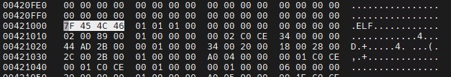
A list of the most popular file signatures can be found at this link.

Binary sectioning

Once a section of the firmware image has been identified, it can be analyzed as a separate file by extracting it with tools such as dd. The dd tool simply copies bytes from an input file to an output file. It is one of the classic tools on Linux systems and has many configuration options.

In some cases, the limits of a section will already have been found, but in others, it will be necessary to define where a file ends. To extract, for example, the ELF executable detected by binwalk at address 0x421000, it is first necessary to determine its size by reading the ELF header at the start address of the file.

Binwalk can do this sectioning and extract the data, but it does not always give satisfactory results, since for many formats it does not calculate total file sizes and simply makes a copy from a signature to the end of the firmware, obtaining better results if the job is done manually.

This sectioning process can be important to be able to split too large firmware into more manageable chunks for further processing or extraction.

Byte distribution

Another analysis that can reveal what use a file may have been a histogram that represents the distribution of values in the file.

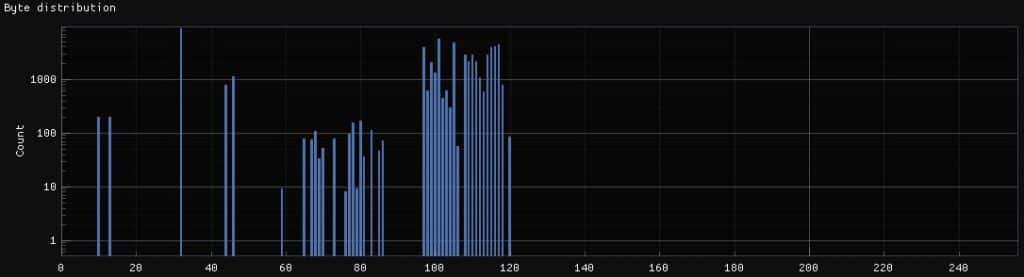
The histogram above shows a widespread use of bytes with values from 97 to 120. To a lesser extent there is also a use of bytes in the range 41 to 86. There is an isolated peak at value 32 and two smaller peaks at values 10 and 13.

This displayed profile matches the usable character distributions in the ASCII table. In particular, the peak at character 32 corresponds to the character representing a blank space, the statistically most used character in plain text.

By profiling the byte distribution of a file, it is possible to recognize different file encodings and even estimate the possible languages in which the text is written.

These same characterizations can occur in binary files or algorithms since, depending on their use, they show a bias in the distribution due to the diverse ways of encoding the information.

String search

Although this is one of the most basic analysis that can be performed, listing the strings inside a file or firmware can provide a lot of information when performing an analysis.

In the case of binary files, strings can display debug messages, software licenses, version messages or even names of functions called from a binary. Knowing what software a binary may be running brings a lot of information to the context in which the analysis is being performed.

It is also common to find strings with compilation dates or firmware packaging, which can provide information on how up-to-date or outdated the firmware is.

$ strings IoTGoat-raspberry-pi2.img
…
console=ttyAMA0,115200 kgdboc=ttyAMA0,115200 console=tty1 root=/dev/mmcblk0p2 rootfstype=ext4 rootwait
…
squashfs: version 4.0 (2009/01/31) Phillip Lougher
…
DTOKLinux version 4.9.152 (embedos@embedos) (gcc version 7.3.0 (OpenWrt GCC 7.3.0 r7676-cddd7b4c77) ) #0 SMP Wed Jan 30 12:21:02 2019
…

Sometimes the strings command may return too much information, so the ‘-n’ parameter is provided to set minimum lengths in the strings it returns.

Search for other constants

Sometimes encrypted sections are identified using entropy analysis, byte distribution or other means. Once such a section is identified, there are not many options to discern whether that section is compressed or encrypted when no signatures are found in them.

In these cases, it is interesting to look for constants in these and other adjacent sections that can guide us in making this identification. Some cryptographic algorithms make use of constant structures to define their initial state. Others are commonly calculated based on tables.

It is common to find the initialization vectors of different hashing algorithms such as MD5, SHA1, SHA256… It is also common to find tables that implement the “Rijndael S-Box” or “AES S-Box” that indicate the use of the AES algorithm, or tables for the calculation of CRC codes, error detection and correction.

Having this information also helps to perform manual analysis using hex editors, as it indicates which integrity checking means have been used to build the firmware image. Thus, if an unknown field is found in a proprietary format and CRC algorithm signatures have been detected, it is interesting to check the most common CRC algorithms as an alternative for the contents of that field.

Manual analysis with a hexadecimal editor

The hex editor is a fundamental tool for analyzing firmware. Although there are many tools available to automate this process, all or many of them rely on heuristics and will require manual supervision.

It is important to evaluate the multiple alternatives for this type of software to find one that the researcher is comfortable with as that investment of time will pay off in the short term.

Different alternatives offer different functionalities that can be especially useful: support for placing markers in a file, structure recognition, entropy analysis, different search engines, CRC calculators, hashes….

This tool is as important as the time spent using it. The investment of time doing these verifications manually can bring great benefits since the experience allows to recognize patterns that many of the automatic tools cannot sense; an important skill that allows to recognize small modifications on known algorithms as a means of obfuscation.

Due to the complexity of analyzing firmware, it is not easy to standardize a single procedure that is valid for all devices. Therefore, the workflow will need to be tailored to each device and will depend heavily on the device manufacturer.

In an analysis, the researcher will have to resort to many of these techniques at quite different times, prioritizing the experience and context acquired during the early stages of the analysis to really be effective in this task.

Experience and the ability to identify the points on which to focus attention at any given time will be important during this phase to conduct an effective analysis.

References:

• https://en.wikipedia.org/wiki/Intel_HEX
• https://en.wikipedia.org/wiki/SREC_(file_format)
• https://en.wikipedia.org/wiki/Hex_dump
• https://en.wikipedia.org/wiki/Base64
• https://hex2bin.sourceforge.net/
• https://srecord.sourceforge.net/
• https://www.micron.com/-/media/client/global/documents/products/data-sheet/nand-flash/20-series/2gb_nand_m29b.pdf
• https://github.com/Hitsxx/NandTool
• https://www.filesignatures.net
• https://en.wikipedia.org/wiki/Entropy_(information_theory)
• https://github.com/OWASP/IoTGoat